Examples of Geomorphometric Analysis (Geomorphometry) Using mapRaster2
Noboru Ogata, Professor Emeritus, Kyoto University
The following pictures show the results of the processing geomorphological data using computers. Computer models of the landform are called Digital Elevation Models (DEM). Although there are several ways of modeling landform, the commonest way of modeling is regularly sampled elevation on the rectangular grid (Grid DEM, aloso known as Altitude Matrix). DEMs are used not only for bird’s eye views of the landform, but also for quantitative analyses of it using computers including derivation of geomorphological variables such as gradient and aspect angle. Research field of these processes is called geomorphometry or digital terrain analysis. The following examples are of 50-meter grid DEM data from the “Sanjō-ga-take” quadrangle in Nara Prefecture supplied by the Geospatial Information Authority of Japan. The study area includes “Sacred Sites and Pilgrimage Routes in the Kii Mountain Range” inscribed on the World Heritage List of UNESCO in July, 2004. Variables are calculated from the DEM data and draped over the surface models in color. To explain the calculation procedures, source codes written in C++ language are provided. For these programs, please take a look at this page.
|
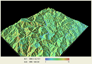
Gradient angle at each location was calculated from the DEM and draped in color.
|
 |
Convexity / Concavity Convexity and concavity (negative convexity) of the terrain are calculated via Laplacian operation. In the study area, where rainfall, surface runoff and streams are dominant factors of terrain formation, index of convexity / concavity shows ridge lines and stream lines. To extract major features of the terrain, the original data are preprocessed by smoothing operation.
|
 |
|
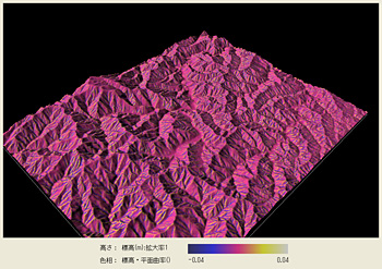
Zevenbergen and Thorne (1987) proposed a procedure to output surface parameters such as slope angle, aspect angle, profile curvature and plan curvature through calculating coefficients of the quadratic surface (polynomial) fitted to the nine neighborhood points. The result of calculating plan curvature is shown on the right. Since the grid of the processed DEM is assumed to be square, the DEM is preprocessed through resampling.
|
 |
|
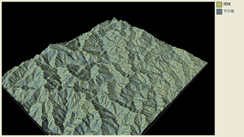
Ridge lines are shown in yellow. The function of extracting ridge lines from DEMs is not implemented in mapRaster2 yet. The program for this function was coded by students at our laboratory using C++ language, based on the procedure described in the pages 54-55 of Principles of Geographical Information Systems for Land Resources Assessment by P. A. Burrough (1986).
|
 |
Stream Lines In the same way as shown above, stream lines are extracted from the DEM and shown in blue. Because of the nature of the Grid DEM, stream lines in the real world cannot be traced exactly. Therefore extracted stream lines are sometimes disconnected.
|
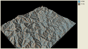 |
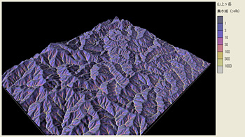
Hydrological Modeling Surface flow from each point on the DEM is simulated, then the flow courses are accumulated to map stream lines. As mentioned above, because of the nature of the Grid DEM, simulated stream lines are sometimes disconnected. The algorithm which approximates the flow by 8 directions (D8 algorithm) might be seen having serious limitation. More important difference of this model from the reality is that, on the forested surface such as this study area, rainfall mostly infiltrates into the soil and does not run over the surface.
|
 |
Last Updated : November 3, 2020
![]()